Airfoil in open jet – Beamforming
This example demonstrates different features of Acoular using measured data from a wind tunnel experiment on trailing edge noise.
It needs the measured timeseries data in example_data.h5 and calibration in example_calib.xml. Both files should reside in the same directory as the example_airfoil_in_open_jet_beamforming.py script.
Note that for a sucessful practical application a much longer timeseries and much finer grid is required.
The script produces three figures:
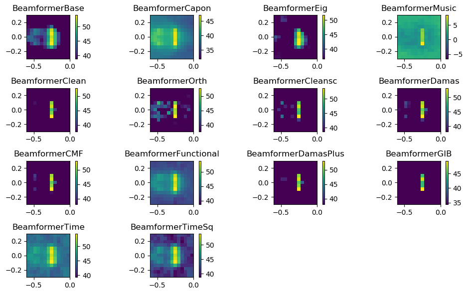
Results for different frequency domain beamformers and averaged time domain beamformers¶ |
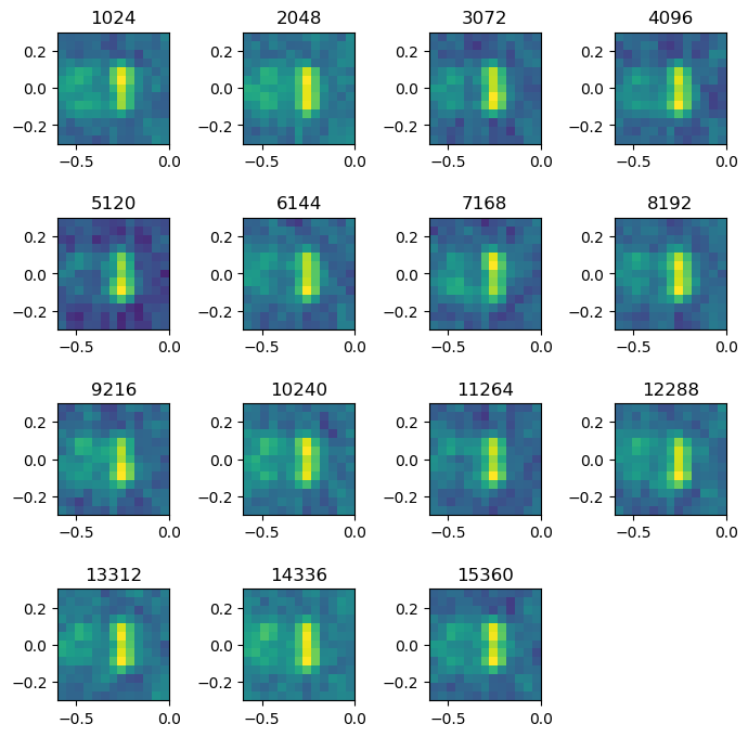
Time domain beamformer output at different times¶ |

Time domain beamformer output with auto-power removal at different times¶ |
# -*- coding: utf-8 -*-
"""
Example "Airfoil in open jet -- Beamforming".

Demonstrates different features of Acoular.

Uses measured data in file example_data.h5,
calibration in file example_calib.xml,
microphone geometry in array_56.xml (part of Acoular).

Copyright (c) 2006-2019 Acoular Development Team.
All rights reserved.
"""

# imports from acoular
import acoular
from acoular import L_p, Calib, MicGeom, Environment, PowerSpectra, \
RectGrid, BeamformerBase, BeamformerEig, BeamformerOrth, BeamformerCleansc, \
MaskedTimeSamples, FiltFiltOctave, BeamformerTimeSq, TimeAverage, \
TimeCache, BeamformerTime, TimePower, BeamformerCMF, \
BeamformerCapon, BeamformerMusic, BeamformerDamas, BeamformerClean, \
BeamformerFunctional, BeamformerDamasPlus, BeamformerGIB, SteeringVector, \
BeamformerCleant,BeamformerCleantSq

# other imports
from numpy import zeros
from os import path
from pylab import figure, subplot, imshow, show, colorbar, title, tight_layout

# files
datafile = 'example_data.h5'
calibfile = 'example_calib.xml'
micgeofile = path.join( path.split(acoular.__file__)[0],'xml','array_56.xml')

#octave band of interest
cfreq = 4000

#===============================================================================
# first, we define the time samples using the MaskedTimeSamples class
# alternatively we could use the TimeSamples class that provides no masking
# of channels and samples
#===============================================================================
t1 = MaskedTimeSamples(name=datafile)
t1.start = 0 # first sample, default
t1.stop = 16000 # last valid sample = 15999
invalid = [1,7] # list of invalid channels (unwanted microphones etc.)
t1.invalid_channels = invalid

#===============================================================================
# calibration is usually needed and can be set directly at the TimeSamples
# object (preferred) or for frequency domain processing at the PowerSpectra
# object (for backwards compatibility)
#===============================================================================
t1.calib = Calib(from_file=calibfile)

#===============================================================================
# the microphone geometry must have the same number of valid channels as the
# TimeSamples object has
#===============================================================================
m = MicGeom(from_file=micgeofile)
m.invalid_channels = invalid

#===============================================================================
# the grid for the beamforming map; a RectGrid3D class is also available
# (the example grid is very coarse)
#===============================================================================
g = RectGrid(x_min=-0.6, x_max=-0.0, y_min=-0.3, y_max=0.3, z=0.68,
             increment=0.05)


#===============================================================================
# the environment, i.e. medium characteristics
# (in this case, the speed of sound is set)
#===============================================================================
env = Environment(c = 346.04)

# =============================================================================
# a steering vector instance. SteeringVector provides the standard freefield
# sound propagation model in the steering vectors.
# =============================================================================
st = SteeringVector(grid=g, mics=m, env=env)

#===============================================================================
# for frequency domain methods, this provides the cross spectral matrix and its
# eigenvalues and eigenvectors, if only the matrix is needed then class
# PowerSpectra can be used instead
#===============================================================================
f = PowerSpectra(time_data=t1,
               window='Hanning', overlap='50%', block_size=128, #FFT-parameters
               ind_low=8, ind_high=16) #to save computational effort, only
               # frequencies with indices 8..15 are used


#===============================================================================
# different beamformers in frequency domain
#===============================================================================
bb = BeamformerBase(freq_data=f, steer=st, r_diag=True)
bc = BeamformerCapon(freq_data=f, steer=st, cached=False)
be = BeamformerEig(freq_data=f, steer=st, r_diag=True, n=54)
bm = BeamformerMusic(freq_data=f, steer=st, n=6)
bd = BeamformerDamas(beamformer=bb, n_iter=100)
bdp = BeamformerDamasPlus(beamformer=bb, n_iter=100)
bo = BeamformerOrth(freq_data=f, steer=st, r_diag=True, eva_list=list(range(38,54)))
bs = BeamformerCleansc(freq_data=f, steer=st, r_diag=True)
bcmf = BeamformerCMF(freq_data=f, steer=st, method='LassoLarsBIC')
bl = BeamformerClean(beamformer=bb, n_iter=100)
bf = BeamformerFunctional(freq_data=f, steer=st, r_diag=False, gamma=4)
bgib = BeamformerGIB(freq_data=f, steer=st, method= 'LassoLars', n=10)

#===============================================================================
# plot result maps for different beamformers in frequency domain
#===============================================================================
figure(1,(10,6))
i1 = 1 #no of subplot
for b in (bb, bc, be, bm, bl, bo, bs, bd, bcmf, bf, bdp, bgib):
    subplot(4,4,i1)
    i1 += 1
    map = b.synthetic(cfreq,1)
    mx = L_p(map.max())
    imshow(L_p(map.T), origin='lower', vmin=mx-15,
           interpolation='nearest', extent=g.extend())
    colorbar()
    title(b.__class__.__name__)

#===============================================================================
# delay and sum beamformer in time domain
# processing chain: beamforming, filtering, power, average
#===============================================================================
bt = BeamformerTime(source=t1, steer=st)
ft = FiltFiltOctave(source=bt, band=cfreq)
pt = TimePower(source=ft)
avgt = TimeAverage(source=pt, naverage = 1024)
cacht = TimeCache( source = avgt) # cache to prevent recalculation

#===============================================================================
# delay and sum beamformer in time domain with autocorrelation removal
# processing chain: zero-phase filtering, beamforming+power, average
#===============================================================================
fi = FiltFiltOctave(source=t1, band=cfreq)
bts = BeamformerTimeSq(source=fi, steer=st, r_diag=True)
avgts = TimeAverage(source=bts, naverage = 1024)
cachts = TimeCache( source = avgts) # cache to prevent recalculation

#===============================================================================
# clean deconvolution in time domain
# processing chain: zero-phase filtering, clean in time domain, power, average
#===============================================================================
fct = FiltFiltOctave(source=t1, band=cfreq)
bct = BeamformerCleant(source=fct, steer=st, n_iter=20,damp=.7)
ptct = TimePower(source=bct)
avgct = TimeAverage(source=ptct, naverage = 1024)
cachct = TimeCache( source = avgct) # cache to prevent recalculation

#===============================================================================
# clean deconvolution in time domain
# processing chain: zero-phase filtering, clean in time domain with
# autocorrelation removal, average
#===============================================================================
fcts = FiltFiltOctave(source=t1, band=cfreq)
bcts = BeamformerCleantSq(source=fcts, steer=st, n_iter=20,damp=.7,r_diag=True)
avgcts = TimeAverage(source=bcts, naverage = 1024)
cachcts = TimeCache( source = avgcts) # cache to prevent recalculation

#===============================================================================
# plot result maps for different beamformers in time domain
#===============================================================================
i2 = 4 # no of figure
for b in (cacht, cachts, cachct, cachcts):
    # first, plot time-dependent result (block-wise)
    figure(i2,(7,7))
    i2 += 1
    res = zeros(g.size) # init accumulator for average
    i3 = 1 # no of subplot
    for r in b.result(1):  #one single block
        subplot(4,4,i3)
        i3 += 1
        res += r[0] # average accum.
        map = r[0].reshape(g.shape)
        mx = L_p(map.max())
        imshow(L_p(map.T), vmax=mx, vmin=mx-15, origin='lower',
               interpolation='nearest', extent=g.extend())
        title('%i' % ((i3-1)*1024))
    res /= i3-1 # average
    tight_layout()
    # second, plot overall result (average over all blocks)
    figure(1)
    subplot(4,4,i1)
    i1 += 1
    map = res.reshape(g.shape)
    mx = L_p(map.max())
    imshow(L_p(map.T), vmax=mx, vmin=mx-15, origin='lower',
           interpolation='nearest', extent=g.extend())
    colorbar()
    title(('BeamformerTime','BeamformerTimeSq','BeamformerCleant',
           'BeamformerCleantSq')[i2-5])
tight_layout()
# only display result on screen if this script is run directly
if __name__ == '__main__': show()