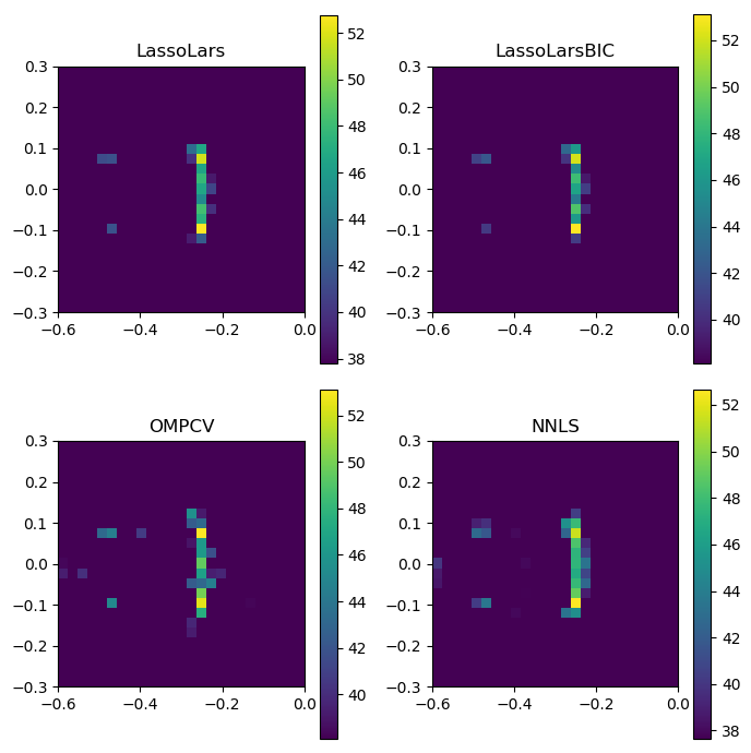
Airfoil in open jet – CMF
Demonstrates CMF methods same setup as in Airfoil in open jet – Beamforming.
It needs the measured timeseries data in example_data.h5 and calibration in example_calib.xml. Both files should reside in the same directory as the example_airfoil_in_open_jet_cmf.py script.
The script produces the figure:
# -*- coding: utf-8 -*-
"""
Example "Airfoil in open jet -- CMF" for Acoular library.

Demonstrates the inverse CMF method with same setup as in example
"Airfoil in open jet -- beamformers".

Uses measured data in file example_data.h5,
calibration in file example_calib.xml,
microphone geometry in array_56.xml (part of Acoular).

Copyright (c) 2006-2019 Acoular Development Team.
All rights reserved.
"""
from __future__ import print_function

# imports from acoular
import acoular
from acoular import L_p, Calib, MicGeom, PowerSpectra, Environment, \
RectGrid, TimeSamples, BeamformerCMF, SteeringVector

# other imports
from os import path
from pylab import figure, subplot, imshow, show, colorbar, title, tight_layout

# files
datafile = 'example_data.h5'
calibfile = 'example_calib.xml'
micgeofile = path.join( path.split(acoular.__file__)[0],'xml','array_56.xml')

#octave band of interest
cfreq = 4000

#===============================================================================
# first, we define the time samples using the MaskedTimeSamples class
# alternatively we could use the TimeSamples class that provides no masking
# of channels and samples
#===============================================================================
t1 = TimeSamples(name=datafile)

#===============================================================================
# calibration is usually needed and can be set directly at the TimeSamples
# object (preferred) or for frequency domain processing at the PowerSpectra
# object (for backwards compatibility)
#===============================================================================
t1.calib = Calib(from_file=calibfile)

#===============================================================================
# the microphone geometry must have the same number of valid channels as the
# TimeSamples object has
#===============================================================================
m = MicGeom(from_file=micgeofile)

#===============================================================================
# the grid for the beamforming map; a RectGrid3D class is also available
# (the example grid is quite coarse)
#===============================================================================
g = RectGrid(x_min=-0.6, x_max=-0.0, y_min=-0.3, y_max=0.3, z=0.68,
             increment=0.025)

#===============================================================================
# the environment, i.e. medium characteristics
# (in this case, the speed of sound is set)
#===============================================================================
env = Environment(c = 346.04)

# =============================================================================
# a steering vector instance. SteeringVector provides the standard freefield
# sound propagation model in the steering vectors.
# =============================================================================
st = SteeringVector(grid=g, mics=m, env=env)

#===============================================================================
# for frequency domain methods, this provides the cross spectral matrix and its
# eigenvalues and eigenvectors, if only the matrix is needed then class
# PowerSpectra can be used instead
#===============================================================================
f = PowerSpectra(time_data=t1,
               window='Hanning', overlap='50%', block_size=256, #FFT-parameters
               ind_low=15, ind_high=31) #to save computational effort, only
               # frequencies with index 15-31 are used

#===============================================================================
# beamformers in frequency domain
#===============================================================================
b = BeamformerCMF(freq_data=f, steer=st, alpha=1e-8)

#===============================================================================
# plot result maps for different beamformers in frequency domain
#===============================================================================
figure(1,(7,7)) #no of figure
i1 = 1 #no of subplot
from time import time
for method in ('LassoLars', 'LassoLarsBIC', 'OMPCV', 'NNLS'):
    b.method = method
    subplot(2,2,i1)
    i1 += 1
    ti = time()
    map = b.synthetic(cfreq,1)
    print(time()-ti)
    mx = L_p(map.max())
    imshow(L_p(map.T), vmax=mx, vmin=mx-15,  origin='lower',
           interpolation='nearest', extent=g.extend())
    colorbar()
    title(b.method)

tight_layout()
# only display result on screen if this script is run directly
if __name__ == '__main__': show()