Note
Go to the end to download the full example code.
Grids#
This example demonstrates the various grid types available in Acoular and their applications in beamforming. We will cover:
Rectangular grids (2D and 3D) for standard beamforming applications
Line grids for analyzing sound sources along a straight line
Grid properties and visualization techniques
Integration with beamforming algorithms
The example includes practical demonstrations of how different grid types affect beamforming results and how to visualize them effectively.
Let’s start by importing the necessary modules.
from pathlib import Path

import acoular as ac
import matplotlib.pyplot as plt
import numpy as np
Measurement Setup#
First, we’ll set up a simulated measurement scenario to demonstrate how grids are used in a typical Acoular workflow. This setup includes:
# Define the microphone array geometry using the standard 64-microphone array stored in an xml file
micgeofile = Path(ac.__file__).parent / 'xml' / 'array_64.xml'
# Create a MicGeom object to represent our microphone geometry
mg = ac.MicGeom(file=micgeofile)
# Deactivate every other microphone
mg.invalid_channels = list(range(0, mg.num_mics, 2))
# Generate simulated time data with three sound sources
pa = ac.demo.create_three_sources_2d(mg, h5savefile='')
# To prepare for beamforming, we need to calculate the frequency spectra (cross spectral matrix)
# of the signals. For this we'll use the PowerSpectra object.
ps = ac.PowerSpectra(source=pa, block_size=128, window='Hanning')
# Next, we'll create a SteeringVector object.
# Steering vectors are crucial for beamforming; they handle the time delays between microphones.
# Keep in mind that the steering vector requires a grid as input, which we'll provide later.
st = ac.SteeringVector(mics=mg)
# Finally, well instantiate a BeamformerBase object.
# This is the foundation for our beamforming algorithms,
# and it takes the frequency data and steering vectors as input.
bb = ac.BeamformerBase(freq_data=ps, steer=st)
Rectangular Grid#
The RectGrid class provides a 2D Cartesian grid for beamforming.
It’s defined by its boundaries in the x-y plane and a constant z-coordinate.
Basic RectGrid usage
Create a rectangular grid in the x-y plane at z = -0.2 m
rg = ac.RectGrid(x_min=-0.2, x_max=0.2, y_min=-0.2, y_max=0.2, z=-0.2, increment=0.01)
Grid Properties
RectGrid provides several useful properties for accessing grid information:
print(f'Grid size: {rg.size}')  # Total number of grid points
print(f'Number of x steps: {rg.nxsteps}')  # Grid points along the x axis
print(f'Number of y steps: {rg.nysteps}')  # Grid points along the y axis
print(f'Grid shape: {rg.shape}')  # (nxsteps, nysteps)
print(f'Grid extent: {rg.extent}')  # Grid boundaries in a format suitable for matplotlib.pyplot's 'imshow' function.
print(f'Grid positions:\n{rg.pos[:, :5]}')  # First 5 grid point positions
Grid size: 1681
Number of x steps: 41
Number of y steps: 41
Grid shape: (41, 41)
Grid extent: (-0.2, 0.2, -0.2, 0.2)
Grid positions:
[[-0.2  -0.2  -0.2  -0.2  -0.2 ]
 [-0.2  -0.19 -0.18 -0.17 -0.16]
 [-0.2  -0.2  -0.2  -0.2  -0.2 ]]
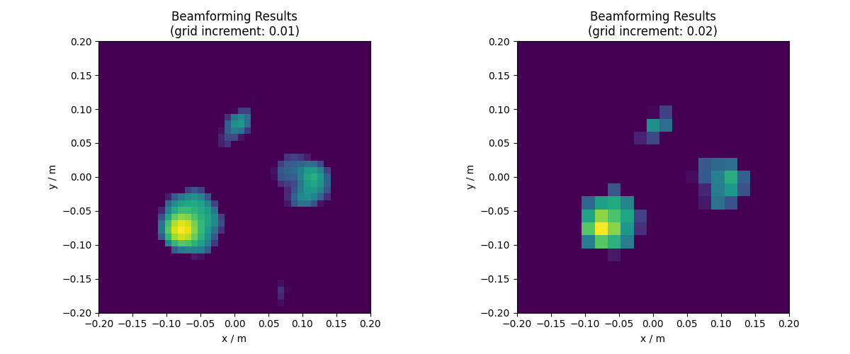
Beamforming with Rectangular Grids
Let’s demonstrate how grid resolution affects beamforming results by varying the grid increment. Before we do this, we need to assign the grid to the steering vector.
st.grid = rg  # Assign the grid to the steering vector

fig = plt.figure(figsize=(12, 5))

# Calculate and plot results for three different grid resolutions
for i in range(2):
    rg.increment = 0.01 * (i + 1)  # Increase grid increment

    # Calculate beamforming output for exactly 8 kHz
    pm = bb.synthetic(8000, 0)
    Lm = ac.L_p(pm)

    # Plot the results
    ax = fig.add_subplot(1, 2, i + 1)
    ax.imshow(
        Lm.T,
        origin='lower',
        vmin=Lm.max() - 10,
        extent=rg.extent,
    )
    ax.set_title(f'Beamforming Results\n(grid increment: {rg.increment})')
    ax.set_xlabel('x / m')
    ax.set_ylabel('y / m')

plt.tight_layout()
plt.show()
[('Mixer_7bd1c67c6bcacd9cee236ed9dbf6bdaa_cache.h5', 1)]
[('Mixer_7bd1c67c6bcacd9cee236ed9dbf6bdaa_cache.h5', 2)]
Note that the results become less precise as the grid increment increases. Conversely, decreasing the grid increment increases the runtime, as more calculations are required. This trade-off between precision and computational cost should be kept in mind for practical applications.
3D Grid#
The RectGrid3D class extends RectGrid to three dimensions,
allowing for volumetric beamforming analysis.
Basic RectGrid3D usage
Create a 3D grid with uniform spacing
rg3d = ac.RectGrid3D(x_min=-0.2, x_max=0.2, y_min=-0.2, y_max=0.2, z_min=-0.3, z_max=-0.1, increment=0.03)

# We can also use different increments for each dimension:
# rg3d.increment = (0.02, 0.02, 0.01)
3D Grid Properties
RectGrid3D provides additional properties for the z-dimension:
print(f'3D Grid size: {rg3d.size}')
print(f'Number of x steps: {rg3d.nxsteps}')
print(f'Number of y steps: {rg3d.nysteps}')
print(f'Number of z steps: {rg3d.nzsteps}')
print(f'3D Grid shape: {rg3d.shape}')
print(f'3D Grid positions:\n{rg3d.pos[:, :5]}')
3D Grid size: 1568
Number of x steps: 14
Number of y steps: 14
Number of z steps: 8
3D Grid shape: (14, 14, 8)
3D Grid positions:
[[-0.2        -0.2        -0.2        -0.2        -0.2       ]
 [-0.2        -0.2        -0.2        -0.2        -0.2       ]
 [-0.3        -0.27142857 -0.24285714 -0.21428571 -0.18571429]]
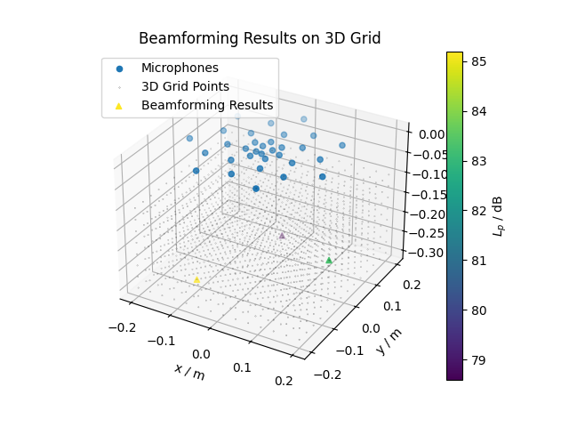
Beamforming with 3D Grids
Let’s demonstrate 3D beamforming using the CLEAN-SC algorithm.
# Generate 3D test data
pa = ac.demo.create_three_sources_3d(mg, h5savefile='')
ps = ac.PowerSpectra(source=pa, block_size=128, window='Bartlett')
bc = ac.BeamformerCleansc(freq_data=ps, steer=st, n_iter=10)

# Update the steering vector with the 3D grid
st.grid = rg3d
rg3d.increment = 0.03  # Set uniform increment
Now we are ready to compute the beamforming output. This time, we’ll calculate it for a frequency of exactly 8 kHz.
map_3d = bc.synthetic(8000, 0)  # Beamformer result in Pa^2
Lm = ac.L_p(map_3d)  # Convert to SPL / dB
# Note that the output of 3D beamforming is a 3D field:
print('3D beamforming output shape:', Lm.shape)
[('/home/runner/work/acoular/acoular/docs/source/auto_examples/cache/Mixer_7bd1c67c6bcacd9cee236ed9dbf6bdaa_cache.h5', 2), ('/home/runner/work/acoular/acoular/docs/source/auto_examples/cache/Mixer_85dd1e5e0ed3372d6ae26b9714b5f01e_cache.h5', 1)]
[('/home/runner/work/acoular/acoular/docs/source/auto_examples/cache/Mixer_7bd1c67c6bcacd9cee236ed9dbf6bdaa_cache.h5', 2), ('/home/runner/work/acoular/acoular/docs/source/auto_examples/cache/Mixer_85dd1e5e0ed3372d6ae26b9714b5f01e_cache.h5', 2)]
3D beamforming output shape: (14, 14, 8)
Visualizing 3D Results
A 3D visualization of the beamforming results can be done in the following way:
fig = plt.figure()
ax = fig.add_subplot(projection='3d')

# Plot microphone positions
ax.scatter(*mg.pos, marker='o', label='Microphones')

# Plot grid points
ax.scatter(*rg3d.pos, s=0.1, c='k', marker='.', label='3D Grid Points')

# Plot beamforming results
indices = Lm > 0
# Find the corresponding grid points to the indices
pos = [p.reshape(Lm.shape)[indices] for p in rg3d.pos]
# Plot the points with color mapping according to their beamforming intensity
scatter = ax.scatter(*pos, c=Lm[indices], marker='^', label='Beamforming Results')

# Add colorbar
cbar = fig.colorbar(scatter)
cbar.set_label('$L_p$ / dB')

# Set labels and title
ax.set(xlabel='x / m', ylabel='y / m', zlabel='z / m')
ax.set_title('Beamforming Results on 3D Grid')
ax.legend(loc='upper left')
plt.show()
Line Grid#
The LineGrid class is useful for analyzing sound sources
along a straight line, such as in pipe flow or for linear machinery.
Basic LineGrid usage
Create a line grid along the x-axis
line_grid = ac.LineGrid()
# We'll start our line at -0.2 meters in the x-direction, with y=0 and z=-0.3 meters
line_grid.loc = (-0.2, 0.0, -0.3)
# The line will point along the x-axis ((1,0,0) being the unit vector in the x-direction)
line_grid.direction = (1.0, 0.0, 0.0)
# Our line will be 40 cm long
line_grid.length = 0.4
# And we'll place 50 points along this line.
line_grid.num_points = 50
Line Grid Properties
Let’s examine the properties of our line grid:
# Let's print out some basic information about our line grid.
print(f'Line grid size: {line_grid.size}')  # Total number of grid points
print(f'Line grid length: {line_grid.length} m')  # Total length of the line
print(f'Number of points: {line_grid.num_points}')  # Number of points along the line
print(f'Start location: {line_grid.loc}')  # Starting point of the line
print(f'Direction vector: {line_grid.direction}')  # Direction of the line
print(f'First 5 grid positions:\n{line_grid.pos[:, :5]}')  # First 5 positions
Line grid size: 50
Line grid length: 0.4 m
Number of points: 50
Start location: (-0.2, 0.0, -0.3)
Direction vector: (1.0, 0.0, 0.0)
First 5 grid positions:
[[-0.2        -0.19183673 -0.18367347 -0.1755102  -0.16734694]
 [ 0.          0.          0.          0.          0.        ]
 [-0.3        -0.3        -0.3        -0.3        -0.3       ]]
Beamforming with Line Grids
Let’s set up a line array measurement scenario.
# Create a line of microphones:
num_mics = 32
pos_total = np.zeros((3, num_mics))
pos_total[0, :] = np.linspace(-0.2, 0.2, num_mics)
line_mg = ac.MicGeom(pos_total=pos_total)

# Generate test data
line_pa = ac.demo.create_three_sources_1d(line_mg, h5savefile='')
ps = ac.PowerSpectra(source=line_pa, block_size=128, window='Hanning')

# Set up beamformer
st.grid = line_grid
st.mics = line_mg
bb = ac.BeamformerBase(freq_data=ps, steer=st)
bs = ac.BeamformerCleansc(freq_data=ps, steer=st)

# Calculate results across full frequency range
freqs = ps.fftfreq()
results = {key: np.zeros((freqs.size, line_grid.num_points)) for key in ['base', 'clean']}

for i, freq in enumerate(freqs):
    results['base'][i, :] = bb.synthetic(freq, 0)
    results['clean'][i, :] = bs.synthetic(freq, 0)
[('/home/runner/work/acoular/acoular/docs/source/auto_examples/cache/Mixer_85dd1e5e0ed3372d6ae26b9714b5f01e_cache.h5', 2), ('/home/runner/work/acoular/acoular/docs/source/auto_examples/cache/Mixer_aa878eb07598abae010071be935c9f79_cache.h5', 1)]
[('/home/runner/work/acoular/acoular/docs/source/auto_examples/cache/Mixer_85dd1e5e0ed3372d6ae26b9714b5f01e_cache.h5', 2), ('/home/runner/work/acoular/acoular/docs/source/auto_examples/cache/Mixer_aa878eb07598abae010071be935c9f79_cache.h5', 2)]
[('/home/runner/work/acoular/acoular/docs/source/auto_examples/cache/Mixer_85dd1e5e0ed3372d6ae26b9714b5f01e_cache.h5', 2), ('/home/runner/work/acoular/acoular/docs/source/auto_examples/cache/Mixer_aa878eb07598abae010071be935c9f79_cache.h5', 3)]
Visualizing Line Grid Results
Create frequency-position plots of the beamforming and source mapping results.
base_levels = ac.L_p(results['base'])
clean_levels = ac.L_p(results['clean'])
vmin = max(base_levels.max(), clean_levels.max()) - 20

fig, (ax1, ax2) = plt.subplots(1, 2, figsize=(12, 5), sharey=True)

mesh1 = ax1.pcolormesh(line_grid.pos[0, :], freqs / 1e3, base_levels, vmin=vmin)
ax1.set_xlabel('Position along line / m')
ax1.set_ylabel('Frequency / kHz')
ax1.set_title('Beamforming Results on Line Grid\n(Base Beamformer)')

mesh2 = ax2.pcolormesh(line_grid.pos[0, :], freqs / 1e3, clean_levels, vmin=vmin)
ax2.set_xlabel('Position along line / m')
ax2.set_title('Source Mapping on Line Grid\n(CLEAN-SC)')

fig.colorbar(mesh1, ax=[ax1, ax2], label='$L_p$ / dB')
plt.show()
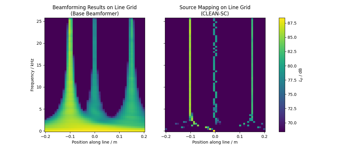
Here, we see the beamforming results of the base beamformer and the source mapping results of the CLEAN-SC algorithm along the line grid. The sources are clearly visible as peaks in the sound pressure level and converge to the source positions in the simulated data for the higher frequencies. Note that the CLEAN-SC algorithm is able to resolve the sources better for lower frequencies than the base beamformer.
Import Grid#
# Define source positions
spos = np.array([[-0.1, -0.1], [0.15, 0], [0, 0.1]])

# Create three grids with bivariate normal distributed points around each source
grids = np.zeros(3, dtype=ac.Grid)
grid_size = 100
for i, p in enumerate(spos):
    gpos = np.zeros((3, grid_size)) - 0.3
    # Generate 100 points with bivariate normal distribution around each source using a small
    # covariance matrix (identity matrix scaled by 1/500) to keep points close to source
    gpos[:2, :] = np.random.multivariate_normal(p, np.eye(2) / 500, size=grid_size).T
    # Create ImportGrid object for each set of points
    grids[i] = ac.ImportGrid(pos=gpos)
The merged grid can be exported to an XML file using the
export_gpos() method.
# grids[0].export_gpos('grid1.xml')
# grids[1].export_gpos('grid2.xml')
# grids[2].export_gpos('grid3.xml')
The XML files can be imported using the file() attribute.
# grid = ac.ImportGrid(file='grid1.xml')
For now, we will create a MergeGrid to combine all three grids and use this merged grid for further processing.
merged_grid = ac.MergeGrid(grids=list(grids))
Let’s visualize the merged grid points.
plt.figure(figsize=(6, 5))
plt.scatter(*merged_grid.pos[:2], c='gray', s=10, label='Grid Points')
plt.scatter(*spos.T, c='r', marker='*', s=200, label='Source Positions')
plt.xlabel('x / m')
plt.ylabel('y / m')
plt.title('Merged Grid with Bivariate Normal Distributed Points')
plt.legend()
plt.grid(True)
plt.show()
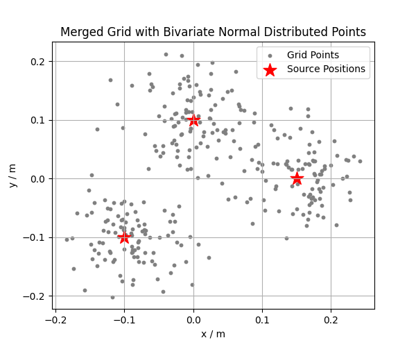
Here, we see the merged grid points distributed around the three source positions. Each source has 100 points following a bivariate normal distribution, creating a cloud of points that is denser near the source and sparser further away.
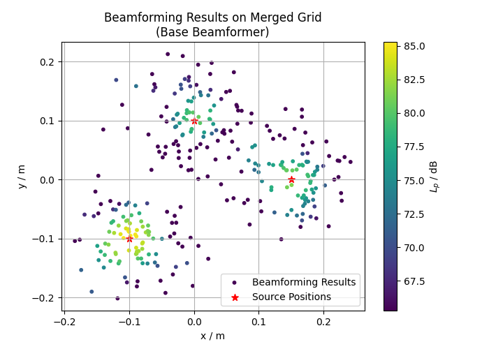
Beamforming with Merged Grid
For beamforming with the merged grid, we return to the measurement setup from the Rectangular Grid and 3D Grid examples.
# Set up the beamformer with the merged grid
pa = ac.demo.create_three_sources_2d(mg, h5savefile='')
ps = ac.PowerSpectra(source=pa, block_size=128, window='Hanning')
st = ac.SteeringVector(grid=merged_grid, mics=mg)
bb = ac.BeamformerBase(freq_data=ps, steer=st)

# Calculate beamforming output for exactly 8 kHz
pm = bb.synthetic(8000, 0)
Lm = ac.L_p(pm)

# Create a scatter plot of the beamforming results
plt.figure(figsize=(7, 5))

s = plt.scatter(*merged_grid.pos[:2], c=Lm, s=10, vmin=Lm.max() - 20, label='Beamforming Results')
plt.scatter(*spos.T, c='r', marker='*', s=50, label='Source Positions')

plt.colorbar(s, label='$L_p$ / dB')
plt.xlabel('x / m')
plt.ylabel('y / m')
plt.title('Beamforming Results on Merged Grid\n(Base Beamformer)')
plt.legend()
plt.grid(True)
plt.show()
[('/home/runner/work/acoular/acoular/docs/source/auto_examples/cache/Mixer_85dd1e5e0ed3372d6ae26b9714b5f01e_cache.h5', 2), ('/home/runner/work/acoular/acoular/docs/source/auto_examples/cache/Mixer_aa878eb07598abae010071be935c9f79_cache.h5', 3), ('/home/runner/work/acoular/acoular/docs/source/auto_examples/cache/Mixer_7bd1c67c6bcacd9cee236ed9dbf6bdaa_cache.h5', 1)]
[('/home/runner/work/acoular/acoular/docs/source/auto_examples/cache/Mixer_85dd1e5e0ed3372d6ae26b9714b5f01e_cache.h5', 2), ('/home/runner/work/acoular/acoular/docs/source/auto_examples/cache/Mixer_aa878eb07598abae010071be935c9f79_cache.h5', 3), ('/home/runner/work/acoular/acoular/docs/source/auto_examples/cache/Mixer_7bd1c67c6bcacd9cee236ed9dbf6bdaa_cache.h5', 2)]
We see that the sound pressure level is highest in the area between the microphones.
See also
Basic Beamforming – Generate a map of three sources.: For basic beamforming concepts
3D Beamforming with CLEAN-SC deconvolution.: For more advanced 3D beamforming applications
Sector Integration Example: For working with grid sectors and integration
Total running time of the script: (0 minutes 7.148 seconds)