Airfoil in open jet – steering vectors.¶

Demonstrates different steering vectors in Acoular and CSM diagonal removal. Uses measured data in file example_data.h5, calibration in file example_calib.xml, microphone geometry in array_56.xml (part of Acoular).

from pathlib import Path

import acoular as ac
from acoular.tools.helpers import get_data_file

The 4 kHz third-octave band is used for the example.

cfreq = 4000
num = 3

Obtain necessary data

time_data_file = get_data_file('example_data.h5')
calib_file = get_data_file('example_calib.xml')

First, we define the time samples using the acoular.sources.MaskedTimeSamples class that provides masking of channels and samples. Here, we exclude the channels with index 1 and 7 and only process the first 16000 samples of the time signals. Alternatively, we could use the acoular.sources.TimeSamples class that provides no masking at all.

t1 = ac.MaskedTimeSamples(file=time_data_file)
t1.start = 0
t1.stop = 16000
invalid = [1, 7]
t1.invalid_channels = invalid

Calibration is usually needed and can be set as a separate processing block with the acoular.Calib object. Invalid channels can be set here as well, by setting the invalid_channels attribute.

calib = ac.Calib(source=t1, file=calib_file, invalid_channels=invalid)

The microphone geometry must have the same number of valid channels as the acoular.sources.MaskedTimeSamples object has. It also must be defined, which channels are invalid.

micgeofile = Path(ac.__file__).parent / 'xml' / 'array_56.xml'
m = ac.MicGeom(file=micgeofile)
m.invalid_channels = invalid

Next, we define a planar rectangular grid for calculating the beamforming map (the example grid is very coarse for computational efficiency). A 3D grid is also available via the acoular.grids.RectGrid3D class.

g = ac.RectGrid(x_min=-0.6, x_max=-0.0, y_min=-0.3, y_max=0.3, z=-0.68, increment=0.05)

For frequency domain methods, acoular.spectra.PowerSpectra provides the cross spectral matrix (and its eigenvalues and eigenvectors). Here, we use the Welch’s method with a block size of 128 samples, Hanning window and 50% overlap.

f = ac.PowerSpectra(source=calib, window='Hanning', overlap='50%', block_size=128)

To define the measurement environment, i.e. medium characteristics, the acoular.environment.Environment class is used. (in this case, only the speed of sound is set)

env = ac.Environment(c=346.04)

The acoular.fbeamform.SteeringVector class provides the standard freefield sound propagation model in the steering vectors.

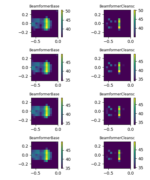
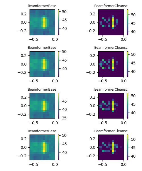
st = ac.SteeringVector(grid=g, mics=m, env=env)

Finally, we define two different beamformers and subsequently calculate the maps for different steering vector formulations. Diagonal removal for the CSM can be performed via the r_diag parameter.

bb = ac.BeamformerBase(freq_data=f, steer=st, r_diag=True)
bs = ac.BeamformerCleansc(freq_data=f, steer=st, r_diag=True)

Plot result maps for different beamformers in frequency domain (left: with diagonal removal, right: without diagonal removal).

import matplotlib.pyplot as plt

fi = 1  # no of figure
for r_diag in (True, False):
    plt.figure(fi, (5, 6))
    fi += 1
    i1 = 1  # no of subplot
    for steer in ('true level', 'true location', 'classic', 'inverse'):
        st.steer_type = steer
        for b in (bb, bs):
            plt.subplot(4, 2, i1)
            i1 += 1
            b.r_diag = r_diag
            map = b.synthetic(cfreq, num)
            mx = ac.L_p(map.max())
            plt.imshow(ac.L_p(map.T), vmax=mx, vmin=mx - 15, origin='lower', interpolation='nearest', extent=g.extent)
            plt.colorbar()
            plt.title(b.__class__.__name__, fontsize='small')

    plt.tight_layout()
    plt.show()

[('example_data_cache.h5', 3)]
[('example_data_cache.h5', 4)]
[('example_data_cache.h5', 5)]

Acoular 25.07 documentation

Airfoil in open jet – steering vectors.

Airfoil in open jet – steering vectors.¶