Beamforming with moving focus

This example demonstrates how to use Acoular to perform moving-focus beamforming with and without CLEANT-based deconvolution for moving sources.

A constellation of four moving white-noise sources passing over a microphone array is evaluated using three different beamforming approaches:

1. Fixed-focus beamforming on a static grid

2. Moving-focus beamforming along a defined trajectory

3. Moving-focus beamforming along the same trajectory with CLEANT-based deconvolution

Setting up the example

At the beginning of this example, we make the necessary imports and define the simulation parameters.

from pathlib import Path

import acoular as ac
import matplotlib.pyplot as plt
import numpy as np

We define the trajectory of the moving focus and the parameters for the moving sources. The trajectory is a straight line along the x-axis at a fixed height (z = 10 m) and y = 0. The sources move at a speed of 60 km/h and pass by the array over a duration of 0.6 seconds.

LX = 5.0  # m, distance to start position on x-axis
LZ = 10.0  # m, distance between array and source plane
V_KMH = 60.0  # km/h, source velocity
VX_M = V_KMH / 3.6  # m/s, source velocity converted to meters per second
T_PASS = 2 * LX / VX_M  # s, total pass-by duration
tr0 = ac.Trajectory(points={0: (-LX, 0, LZ), T_PASS: (LX, 0, LZ)})  # moving focus trajectory

Next, we define parameters for the microphone array, the processing blocks, and the frequency band of interest.

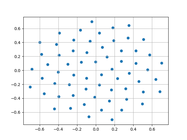
The example uses a 64-microphone array.

mics = ac.MicGeom(file=Path(ac.__file__).parent / 'xml' / 'tub_vogel64.xml')
plt.scatter(*mics.pos[:2])
plt.grid()

The sampling frequency is set to 6.4 kHz, and the total number of samples is calculated based on the pass duration.

SFREQ = 6400  # Hz, sampling frequency
NUM_SAMPLES = int(T_PASS * SFREQ)  # total number of samples

The processing block size is set to 1/4 of the total number of samples.

BLOCK_SIZE = int(NUM_SAMPLES / 4)  # number of samples per processing block

The frequency band of interest is set to 2000 Hz, which corresponds to a third-octave band used for analysis.

FREQ = 2000  # Hz, third-octave band used for analysis

Beamforming will be performed using a rectangular grid in the x-y plane, centered at the origin (0, 0) and extending from -2 to 2 meters in both x and y directions. The grid increment is set to 0.2 meters for faster computation.

Generally, Acoular works with dimensionless units, but since we defined the trajectory in meters above, we will use the same unit for the grid.

rg = ac.RectGrid(x_min=-2, x_max=2, y_min=-2, y_max=2, z=0, increment=0.2)

The steering vector is created for the grid and the microphone array. This vector is used to steer the beamformer towards the desired focus trajectory.

st = ac.SteeringVector(grid=rg, mics=mics)

The WNoiseGenerator is used to create white-noise signal generators for the sources. Each source has a different root mean square (RMS) value, which is set to 0.564 multiplied by a factor that decreases with each source.

def wngen(nseed):
    rms = 0.564 * 10 ** (-0.5 * (nseed - 1))
    return ac.WNoiseGenerator(sample_freq=SFREQ, num_samples=NUM_SAMPLES, seed=nseed, rms=rms)


sigs = [wngen(1 + i) for i in range(4)]

The four sources are positioned at the corners of a square spanning an area of 2 by 2 meters. For each source position, a trajectory is created that is offset from the moving focus trajectory. The sources move linearly along the x-axis, passing by the microphone array.

source_pos = [(1, 1, 0), (1, -1, 0), (-1, -1, 0), (-1, 1, 0)]


def create_trajectory(x, y, z):
    # Linear trajectory offset by source position
    return ac.Trajectory(points={0: (-LX + x, y, LZ + z), T_PASS: (LX + x, y, LZ + z)})


trs = [create_trajectory(*sp) for sp in source_pos]

The sources are combined with their respective trajectories using the MovingPointSource class. The conv_amp parameter is set to True to account for amplitude changes due to distance variations.

mps = [
    ac.MovingPointSource(signal=sig, mics=mics, trajectory=tr, conv_amp=True) for sig, tr in zip(sigs, trs, strict=True)
]

Finally, the sources are mixed together using the SourceMixer class. This class combines the individual source signals into a single mixed signal that can be processed further down the chain.

source_mixer = ac.SourceMixer(sources=mps)

On top of these preparations for the moving sources and trajectory, we also define a visualization function to plot the beamforming maps.

def plot_maps(res, grid, figure_title):
    n = 3
    fig, axes = plt.subplots(1, n, figsize=(12, 4), sharey=True, layout='constrained')
    times = [(i * BLOCK_SIZE) / SFREQ for i in range(n)]
    res = ac.L_p(res)
    mx = res.max()
    for ax, r, t in zip(axes, res, times, strict=True):
        r0 = r.reshape(grid.shape).T
        im = ax.imshow(
            r0,
            origin='lower',
            vmax=mx,
            vmin=mx - 15,
            interpolation='nearest',
            extent=grid.extent,
            cmap='viridis',
        )
        ax.set_title(f'$t$ = {t:.2f} s')
        ax.set_xlabel('$x$ in m')

    axes[0].set_ylabel('$y$ in m')
    fig.subplots_adjust(wspace=0.075)
    fig.colorbar(im, ax=axes.ravel(), pad=0.04, label='$L_p$ in dB')

    if figure_title:
        fig.suptitle(figure_title)
    plt.show()

Beamforming in the time domain with fixed focus

Before we compute the moving-focus beamforming maps, we first perform time-domain beamforming with a fixed focus on a larger grid. This serves as a baseline to compare against the moving-focus results.

For the fixed-focus case, the grid is placed at z = LZ, i.e., in the plane of the sources, while the moving-focus grid follows the trajectory tr0 at z = 0 (in the plane of the microphones). It is also wider in the x direction to account for the source movement during the pass-by.

rg_fixed = ac.RectGrid(x_min=-3, x_max=3, y_min=-2, y_max=2, z=LZ, increment=0.2)
st_fixed = ac.SteeringVector(grid=rg_fixed, mics=mics)

We now connect the processing blocks into a chain that can be executed by Acoular. The chain is:

We already have the first block, SourceMixer, defined as source_mixer. The subsequent blocks are:

1. FiltFiltOctave: zero-phase third-octave filtering around FREQ.

2. BeamformerTimeSq: computes (squared) beamforming.

3. Average: groups frames into blocks of BLOCK_SIZE samples to produce one map per block.

4. Cache: stores the averaged maps so that repeated access is fast and deterministic.

This processing chain is similar to the one used later for moving-focus beamforming.

fi_fixed = ac.FiltFiltOctave(source=source_mixer, band=FREQ, fraction='Third octave')
bt_fixed = ac.BeamformerTimeSq(source=fi_fixed, steer=st_fixed, r_diag=True)
avgt_fixed = ac.Average(source=bt_fixed, num_per_average=BLOCK_SIZE)
cacht_fixed = ac.Cache(source=avgt_fixed)

In the following step, we execute the processing chain and retrieve a small number of averaged beamforming maps for visualization.

The num argument controls how many averaged blocks to return. Use num=None to return all cached blocks, or set num to an integer to limit the number of returned maps.

res_fixed = next(cacht_fixed.result(num=3))
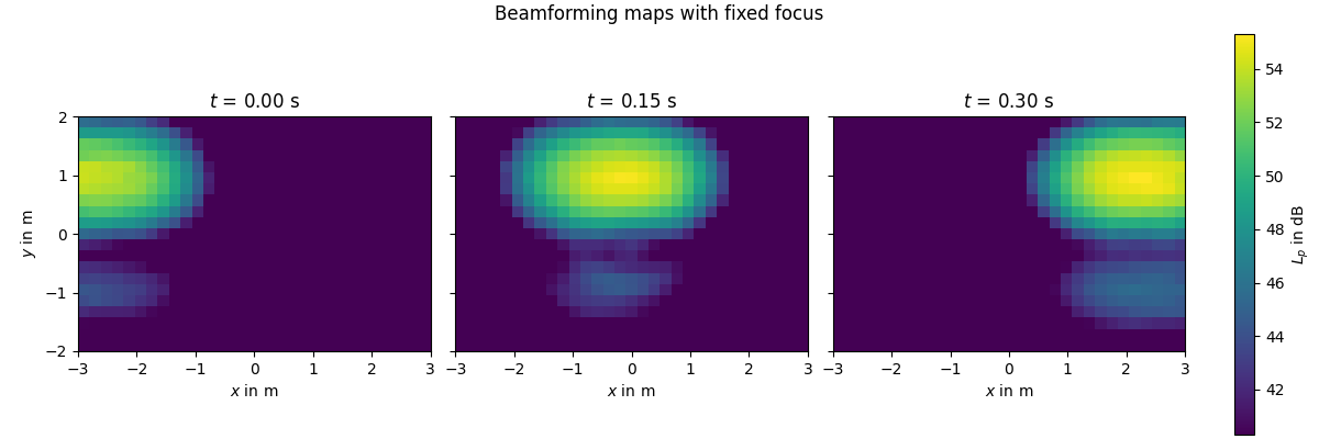
plot_maps(res_fixed, rg_fixed, figure_title='Beamforming maps with fixed focus')

[('void_cache.h5', 1)]
/home/runner/work/acoular/acoular/examples/moving_sources_examples/example_beamforming_with_moving_focus.py:165: UserWarning: This figure was using a layout engine that is incompatible with subplots_adjust and/or tight_layout; not calling subplots_adjust.
  fig.subplots_adjust(wspace=0.075)

In the above plot, we observe that the fixed-focus beamforming maps show the sources as they pass by the microphone array. However, due to the fixed focus and the averaging, the spatial resolution is limited, and the sources appear blurred as they move across the grid.

Beamforming in the time domain with moving focus

Now for the main part of this example: compute time-domain beamforming maps along a moving focus trajectory tr0. The focus follows the provided trajectory while beamforming on the grid rg.

We now connect the processing blocks into a chain that can be executed by Acoular. The chain is:

fi_mov = ac.FiltFiltOctave(source=source_mixer, band=FREQ, fraction='Third octave')
bt_mov = ac.BeamformerTimeSqTraj(source=fi_mov, steer=st, trajectory=tr0, r_diag=True)
avgt_mov = ac.Average(source=bt_mov, num_per_average=BLOCK_SIZE)
cacht_mov = ac.Cache(source=avgt_mov)

res_mov = next(cacht_mov.result(num=3))
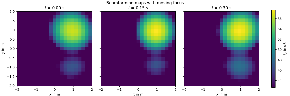
plot_maps(res_mov, rg, figure_title='Beamforming maps with moving focus')

[('void_cache.h5', 2)]

In the moving-focus beamforming maps, we see that the sources are better localized as they pass by the microphone array. The moving focus allows the beamformer to track the sources more effectively, resulting in improved spatial resolution compared to the fixed-focus case.

Beamforming with deconvolution (CLEANT) in the time domain with moving focus

Finally, we apply CLEANT-based deconvolution while beamforming along the same moving focus trajectory. This improves spatial resolution and reduces sidelobes. The processing chain is similar to the previous one, but we replace BeamformerTimeSqTraj with BeamformerCleantSqTraj.

fi_cleant = ac.FiltFiltOctave(source=source_mixer, band=FREQ, fraction='Third octave')
bt_cleant = ac.BeamformerCleantSqTraj(source=fi_cleant, steer=st, trajectory=tr0, conv_amp=True)
avgt_cleant = ac.Average(source=bt_cleant, num_per_average=BLOCK_SIZE)
cacht_cleant = ac.Cache(source=avgt_cleant)

res_cleant = next(cacht_cleant.result(num=3))
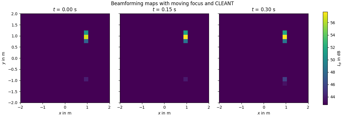
plot_maps(res_cleant, rg, figure_title='Beamforming maps with moving focus and CLEANT')

[('void_cache.h5', 3)]

In the moving-focus beamforming maps with CLEANT, we observe a significant improvement in spatial resolution compared to both the fixed-focus and moving-focus without CLEANT cases. The sources are more sharply defined, and the sidelobes are reduced, demonstrating the effectiveness of CLEANT deconvolution in enhancing beamforming results for moving sources.