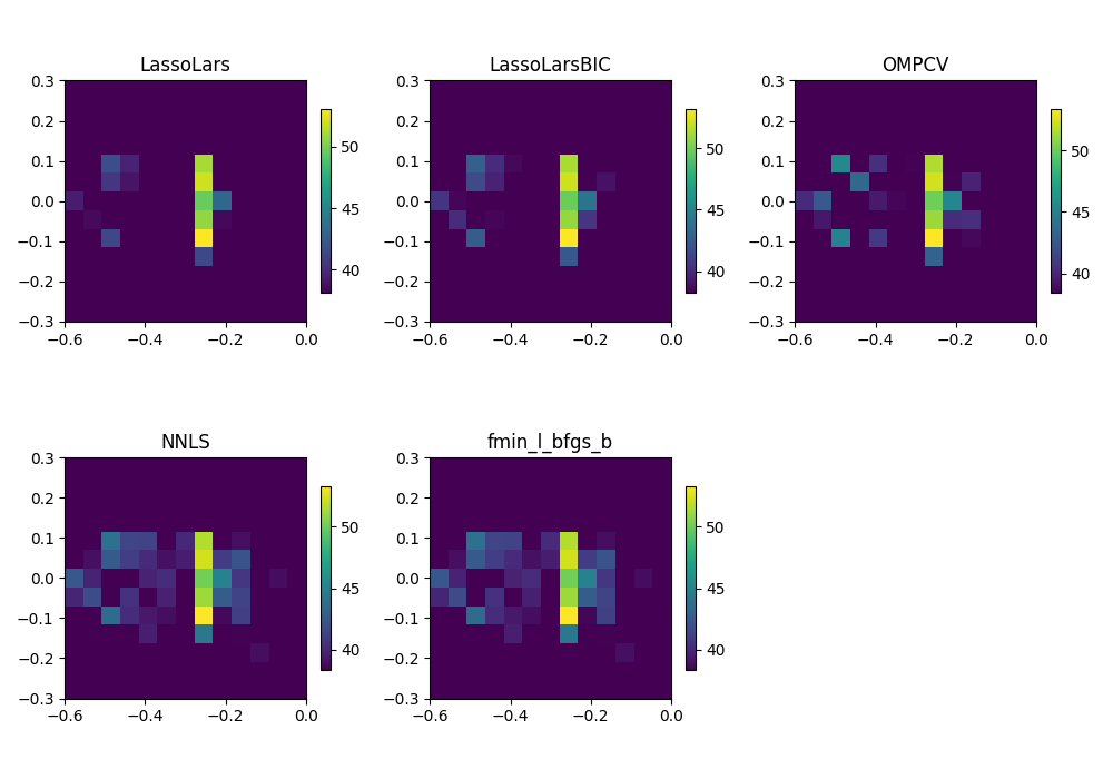
Airfoil in open jet – Covariance matrix fitting (CMF).¶

Demonstrates the inverse CMF method with different solvers. Uses measured data in file example_data.h5, calibration in file example_calib.xml, microphone geometry in array_56.xml (part of Acoular).

from pathlib import Path

import acoular as ac
from acoular.tools.helpers import get_data_file

The 4 kHz third-octave band is used for the example.

cfreq = 4000
num = 3

Obtain necessary data

time_data_file = get_data_file('example_data.h5')
calib_file = get_data_file('example_calib.xml')

Setting up the processing chain for acoular.fbeamform.BeamformerCMF methods.

Hint

A step-by-step explanation for setting up the processing chain is given in the example Airfoil in open jet – steering vectors..

ts = ac.MaskedTimeSamples(
    file=time_data_file,
    invalid_channels=[1, 7],
    start=0,
    stop=16000,
)
calib = ac.Calib(source=ts, file=calib_file, invalid_channels=[1, 7])
mics = ac.MicGeom(file=Path(ac.__file__).parent / 'xml' / 'array_56.xml', invalid_channels=[1, 7])
grid = ac.RectGrid(x_min=-0.6, x_max=-0.0, y_min=-0.3, y_max=0.3, z=-0.68, increment=0.05)
env = ac.Environment(c=346.04)
st = ac.SteeringVector(grid=grid, mics=mics, env=env)
f = ac.PowerSpectra(source=calib, window='Hanning', overlap='50%', block_size=128)
b = ac.BeamformerCMF(freq_data=f, steer=st, alpha=1e-8)

Plot result maps for CMF with different solvers from SciPy and scikit-learn, including:

LassoLars
LassoLarsBIC
OMPCV
NNLS
fmin_l_bfgs_b

import matplotlib.pyplot as plt

plt.figure(1, (10, 7))  # no of figure
i1 = 1  # no of subplot

for method in ('LassoLars', 'LassoLarsBIC', 'OMPCV', 'NNLS', 'fmin_l_bfgs_b'):
    b.method = method
    plt.subplot(2, 3, i1)
    i1 += 1
    map = b.synthetic(cfreq, 1)
    mx = ac.L_p(map.max())
    plt.imshow(ac.L_p(map.T), vmax=mx, vmin=mx - 15, origin='lower', interpolation='nearest', extent=grid.extent)
    plt.colorbar(shrink=0.5)
    plt.title(b.method)

plt.tight_layout()
plt.show()

LassoLars, LassoLarsBIC, OMPCV, NNLS, fmin_l_bfgs_b

[('example_data_cache.h5', 1)]
[('example_data_cache.h5', 2)]

Total running time of the script: (0 minutes 4.409 seconds)

Gallery generated by Sphinx-Gallery

Acoular 25.07 documentation

Airfoil in open jet – Covariance matrix fitting (CMF).

Airfoil in open jet – Covariance matrix fitting (CMF).¶