MultiSector

This example demonstrates how to use the MultiSector class in Acoular to combine multiple sectors and perform spatial integration over complex regions. It reuses the measurement setup and helper functions from the sectors example for convenience.

Preparation

First, we import the modules and functions we are going to use in this example.

from pathlib import Path

import acoular as ac
import matplotlib.pyplot as plt
import numpy as np
from acoular.tools import barspectrum
from acoular.tools.helpers import get_data_file

# Import Acoular objects and helper functions from the sectors example
# from example_sectors import bb, freqs, grid, sector, spl_map

time_data_file = get_data_file('example_data.h5')
calib_file = get_data_file('example_calib.xml')

ts = ac.MaskedTimeSamples(
    file=time_data_file,
    invalid_channels=[1, 7],
    start=0,
    stop=16000,
)
calib = ac.Calib(source=ts, file=calib_file, invalid_channels=[1, 7])
mics = ac.MicGeom(file=Path(ac.__file__).parent / 'xml' / 'array_56.xml', invalid_channels=[1, 7])
grid = ac.RectGrid(x_min=-0.6, x_max=0.0, y_min=-0.3, y_max=0.3, z=-0.68, increment=0.05)
env = ac.Environment(c=346.04)
st = ac.SteeringVector(grid=grid, mics=mics, env=env)
f = ac.PowerSpectra(source=calib, window='Hanning', overlap='50%', block_size=128)
bb = ac.BeamformerBase(freq_data=f, steer=st)

sector = ac.RectSector(x_min=-0.275, x_max=-0.225, y_min=-0.20, y_max=0.15)

map = bb.synthetic(8000)
spl_map = ac.L_p(map)

freqs = f.fftfreq()

[('example_data_cache.h5', 1)]
[('example_data_cache.h5', 2)]

Combining Sectors

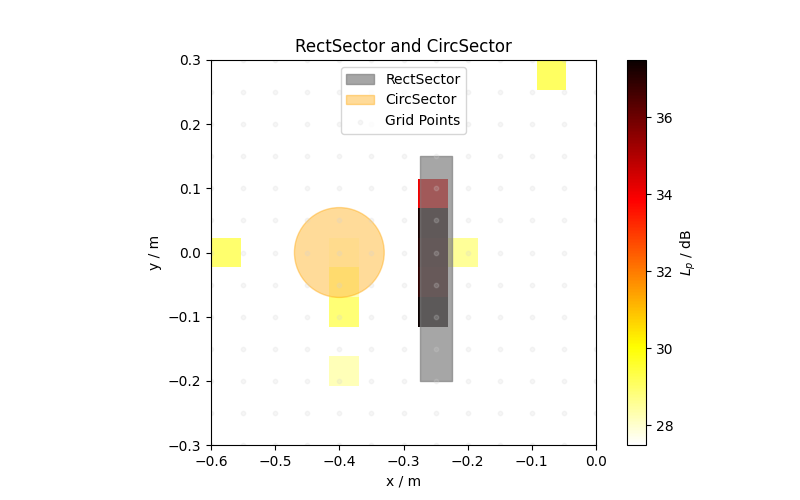
Since the MultiSector class combines multiple Sector-derived objects, we need to define a second sector. Here, we choose the CircSector class.

circsector = ac.CircSector(x=-0.4, y=0.0, r=0.07)

Let us see how the two sectors look on the source map.

plt.figure(figsize=(8, 5))
im = plt.imshow(spl_map.T, origin='lower', vmin=spl_map.max() - 10, extent=grid.extent, cmap='hot_r')
plt.fill_between([sector.x_min, sector.x_max], sector.y_min, sector.y_max, alpha=0.7, label='RectSector', color='gray')
circ = plt.Circle((circsector.x, circsector.y), circsector.r, color='orange', alpha=0.4, label='CircSector')
plt.gca().add_patch(circ)
plt.scatter(*grid.pos[0:2], c='lightgray', s=10, label='Grid Points', alpha=0.2)
plt.xlabel('x / m')
plt.ylabel('y / m')
plt.title('RectSector and CircSector')
plt.colorbar(im, label='$L_p$ / dB')
plt.legend()
plt.show()

Now we create a MultiSector object that encompasses both sectors.

multisector = ac.MultiSector(sectors=[sector, circsector])

Note that this object does not have the attributes of the SingleSector class: The include_border, abs_tol, and default_nearest attributes are not part of the MultiSector class.

Integrate Over the MultiSector

Here, as in the sector example, we integrate once over all FFT frequencies and then also look at the third-octova spectrum.

# Define a function to get only SPL spectrum values greater than zero
def get_spl(spectrum):
    spl = ac.L_p(spectrum)
    return np.where(spl > 0, spl, 0)


# Integrate over multisector
bf_multisector = bb.integrate(multisector)

# Use barspectrum to get third-octave bands
f_borders, bars, f_center = barspectrum(bf_multisector, freqs, 3, bar=True)


fig, ax1 = plt.subplots(figsize=(10, 6))
color1 = 'tab:blue'
color2 = 'tab:orange'

ax1.set_xlabel('Frequency / Hz')
ax1.fill_between(f_borders, get_spl(bars), color=color2, alpha=0.5, label='Third-Octave Barspectrum')
ax1.set_ylabel('$L_p$ / dB', color=color1)
ax1.tick_params(axis='y', labelcolor=color1)
ax1.set_title('MultiSector Integration: Spectrum and Third-Octave Barspectrum')
ax1.grid(True)

ax2 = ax1.twinx()
ax2.plot(freqs, get_spl(bf_multisector), color=color1, label='Integrated Spectrum (all freqs)')
ax2.set_ylabel('$L_p$ / dB (barspectrum)', color=color2)
ax2.tick_params(axis='y', labelcolor=color2)
ax2.set_ylim(ax1.get_ylim())
ax2.set_xscale('log')

fig.tight_layout()
fig.legend(loc='upper right', bbox_to_anchor=(0.93, 0.93))
plt.show()

/home/runner/work/acoular/acoular/acoular/tools/helpers.py:213: Warning: Queried frequency band (445.449 to 561.231 Hz) does not include any discrete FFT sample frequencies. Returning zeros.
  p = np.array([synthetic(data, fftfreqs, list(fc[i_low:i_high]), num)])
/home/runner/work/acoular/acoular/acoular/tools/helpers.py:213: Warning: Queried frequency band (561.266 to 707.151 Hz) does not include any discrete FFT sample frequencies. Returning zeros.
  p = np.array([synthetic(data, fftfreqs, list(fc[i_low:i_high]), num)])
/home/runner/work/acoular/acoular/acoular/tools/helpers.py:213: Warning: Queried frequency band (890.899 to 1122.46 Hz) does not include any discrete FFT sample frequencies. Returning zeros.
  p = np.array([synthetic(data, fftfreqs, list(fc[i_low:i_high]), num)])

You can use MultiSector with any combination of sector types, such as RectSector, CircSector, and PolySector. This makes it easy to analyze complex regions in your sound field.