Sectors

This example demonstrates how to use a sector for spatial integration in Acoular. It uses the airfoil-in-open-jet dataset, places a rectangular sector on the trailing edge of the airfoil, integrates the beamforming result over this sector, and plots the normal and the third-octave spectra using the barspectrum() function.

Preparation

First, we import the modules and functions we are going to use in this example.

from pathlib import Path

import acoular as ac
import matplotlib.pyplot as plt
import numpy as np
from acoular.tools import barspectrum
from acoular.tools.helpers import get_data_file

Next, let’s ensure we have the necessary example data available.

The calibration and measurement files will be downloaded automatically if they are not already present.

# Download example data if necessary
time_data_file = get_data_file('example_data.h5')
calib_file = get_data_file('example_calib.xml')

invalid = [1, 7]  # Invalid channels for this dataset
ts = ac.MaskedTimeSamples(
    file=time_data_file,
    invalid_channels=invalid,
    start=0,
    stop=16000,
)
calib = ac.Calib(source=ts, file=calib_file, invalid_channels=invalid)
mics = ac.MicGeom(file=Path(ac.__file__).parent / 'xml' / 'array_56.xml', invalid_channels=invalid)
grid = ac.RectGrid(x_min=-0.6, x_max=0.0, y_min=-0.3, y_max=0.3, z=-0.68, increment=0.05)
env = ac.Environment(c=346.04)
st = ac.SteeringVector(grid=grid, mics=mics, env=env)
f = ac.PowerSpectra(source=calib, window='Hanning', overlap='50%', block_size=128)
bb = ac.BeamformerCleansc(freq_data=f, steer=st)

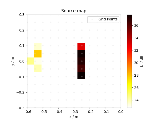
The microphone array captures the acoustic signature of an airfoil positioned in an open jet. The resulting source map, computed via source mapping at 8 kHz, is displayed below.

# Calculate the power map for 8 kHz
pm = bb.synthetic(8000)
spl_pm = ac.L_p(pm)

# Display source mapping results for 8 kHz
plt.scatter(*grid.pos[0:2], c='lightgray', s=10, label='Grid Points', alpha=0.2)
plt.imshow(spl_pm.T, vmax=spl_pm.max(), vmin=spl_pm.max() - 15, origin='lower', extent=grid.extent, cmap='hot_r')

cbar = plt.colorbar()
cbar.set_label('$L_p$ / dB')
plt.xlabel('x / m')
plt.ylabel('y / m')
plt.title('Source map')
plt.legend()
plt.show()

[('example_data_cache.h5', 3)]
[('example_data_cache.h5', 4)]

The trailing edge of an airfoil is often a region of particular acoustic interest. To investigate this area more closely, we will utilize Acoular’s sector classes.

Define a Sector

Let us start by defining a sector.

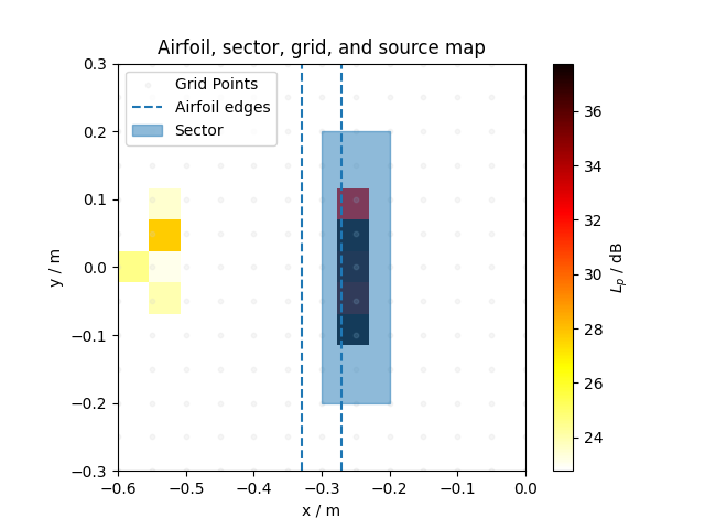
With a sector, spatial integrations of the individual source contributions of interest can be performed after calculating the full source map. Here, we will create a rectangular sector that covers the trailing edge of the airfoil.

sector = ac.RectSector(x_min=-0.3, x_max=-0.2, y_min=-0.2, y_max=0.2)

To see how our sector and airfoil look together, we visulaize the airfoil’s front and trailing edges (as dashed lines), the sector (as a light blue rectangle), and the grid points (where the sound field is calculated). This helps us see exactly what region we are integrating over later.

plt.scatter(*grid.pos[0:2], c='lightgray', s=10, label='Grid Points', alpha=0.2)
# Plot airfoil's edges as dashed lines (we assume they are at x = -0.3 and x = -0.25)
plt.vlines([-0.33, -0.27], ymin=-0.3, ymax=0.3, linestyles='--', label='Airfoil edges')
# Plot sector as a filled rectangle
plt.fill_between([sector.x_min, sector.x_max], sector.y_min, sector.y_max, alpha=0.5, label='Sector', color='C0')
plt.imshow(spl_pm.T, vmax=spl_pm.max(), vmin=spl_pm.max() - 15, origin='lower', extent=grid.extent, cmap='hot_r')

cbar = plt.colorbar()
cbar.set_label('$L_p$ / dB')
plt.xlabel('x / m')
plt.ylabel('y / m')
plt.title('Airfoil, sector, grid, and source map')
plt.legend()
plt.show()

Grid Points of Interest

Acoular’s sector classes define regions of interest on the grid. Each sector provides a contains() method that accepts a grid’s pos attribute and determines which grid points fall within the sector.

For a grid with N points, the contains() method returns a boolean mask of length N, where True indicates points inside the sector.

mask = sector.contains(grid.pos)
print('x: {}\ny: {}'.format(*grid.pos[:2, mask]))
print(mask)

x: [-0.3  -0.3  -0.3  -0.3  -0.3  -0.3  -0.3  -0.3  -0.3  -0.25 -0.25 -0.25
 -0.25 -0.25 -0.25 -0.25 -0.25 -0.25 -0.2  -0.2  -0.2  -0.2  -0.2  -0.2
 -0.2  -0.2  -0.2 ]
y: [-0.2  -0.15 -0.1  -0.05  0.    0.05  0.1   0.15  0.2  -0.2  -0.15 -0.1
 -0.05  0.    0.05  0.1   0.15  0.2  -0.2  -0.15 -0.1  -0.05  0.    0.05
  0.1   0.15  0.2 ]
[False False False False False False False False False False False False
 False False False False False False False False False False False False
 False False False False False False False False False False False False
 False False False False False False False False False False False False
 False False False False False False False False False False False False
 False False False False False False False False False False False False
 False False False False False False False False  True  True  True  True
  True  True  True  True  True False False False False  True  True  True
  True  True  True  True  True  True False False False False  True  True
  True  True  True  True  True  True  True False False False False False
 False False False False False False False False False False False False
 False False False False False False False False False False False False
 False False False False False False False False False False False False
 False False False False False False False False False False False False
 False]

We observe 27 grid points marked as True in the mask: 7 points strictly inside the sector and 20 additional points lying on its borders. To exclude points on the border, we can set the sector’s include_border attribute to False.

Additionally, the tolerance for determining whether a grid point lies on the sector’s border can be adjusted via the abs_tol attribute.

sector.include_border = False
mask = sector.contains(grid.pos)
print('x: {}\ny: {}'.format(*grid.pos[:2, mask]))

x: [-0.25 -0.25 -0.25 -0.25 -0.25 -0.25 -0.25]
y: [-0.15 -0.1  -0.05  0.    0.05  0.1   0.15]

Now, only seven points are strictly inside the sector. They all lie on the x-position -0.25, with y-values -0.15, -0.1, -0.05, 0.0, 0.05, 0.1, and 0.15.

For sectors that contain no grid points (neither inside nor on the borders), the default_nearest attribute can be used. When set to True, as it is by default, and if the sector contains no grid points, it selects the grid point closest to the sector’s center. When set to False, no points will be selected.

The grid points identified by the sector determine which points are integrated over using the beamformer’s integrate() method or Acoular’s integrate() function.

Integrate Over Sector

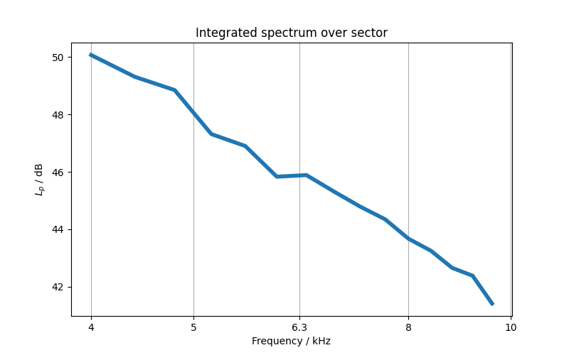
Now for the main event: integrating the beamforming result over our sector. This step gives us the total sound pressure level (SPL) coming from just our region of interest. We can use the beamformer’s integrate() method and Acoular’s L_p() function to get SPL associated with the sector.

Calculation the result for all frequencies can be computationally expensive and highly inefficient, especially for large datasets. Instead of using all FFT frequencies provided by the PowerSpectra object, we can limit the frequency range to focus on a specific band of interest.

This can be achieved either by setting the ind_low and ind_high attributes, or by passing a frequency range directly to the integrate() method or integrate() function. Here, we will use the latter approach to integrate over the frequency range from 4 kHz to 10 kHz.

freqs, bf_sector = bb.integrate(sector, frange=(4000, 10000))
spl_sector = ac.L_p(bf_sector)
spl_sector = np.where(spl_sector > 0, spl_sector, 0)  # Keep positive entries only

plt.figure(figsize=(8, 5))
plt.semilogx(freqs, spl_sector, color='C0', linewidth=4)
plt.xticks([4000, 5000, 6300, 8000, 10000], labels=['4', '5', '6.3', '8', '10'])

plt.xlabel('Frequency / kHz')
plt.ylabel('$L_p$ / dB')
plt.title('Integrated spectrum over sector')
plt.grid(which='major', axis='x')
plt.minorticks_off()
plt.show()

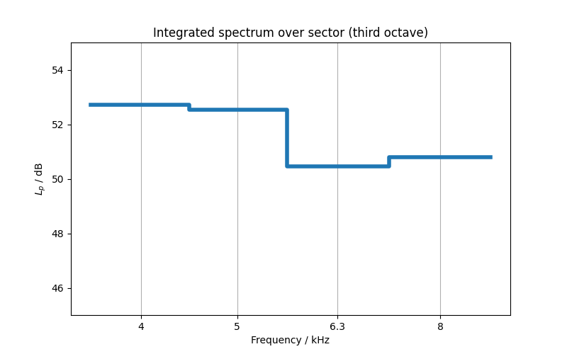
Third-Octave Barspectrum

Using Acoular’s barspectrum() function we can easily convert our integrated spectrum into third-octave bands.

f_borders, bars, f_center = barspectrum(bf_sector, freqs, 3, bar=True)
spl_bars = ac.L_p(bars)

plt.figure(figsize=(8, 5))
plt.plot(f_borders, spl_bars, color='C0', linewidth=4)
plt.ylim(45, 55)
plt.xscale('log')
plt.xticks(f_center, labels=['4', '5', '6.3', '8'])

plt.xlabel('Frequency / kHz')
plt.ylabel('$L_p$ / dB')
plt.title('Integrated spectrum over sector (third octave)')
plt.grid(which='major', axis='x')
plt.minorticks_off()
plt.show()

Other Sectors

Acoular provides several other sector types for flexible spatial integration:

• RectSector: Rectangle in the x-y plane (as used above).

• CircSector: Circular sector in the x-y plane.

• PolySector: Arbitrary polygonal sector in the x-y plane.

• ConvexSector: Convex hull sector in the x-y plane.

• RectSector3D: 3D cuboid sector (for 3D grids).

• MultiSector: Combines multiple sectors of any type.

All sector types can be used with the integrate function to sum or average results over the selected region.